Interest Rate Models

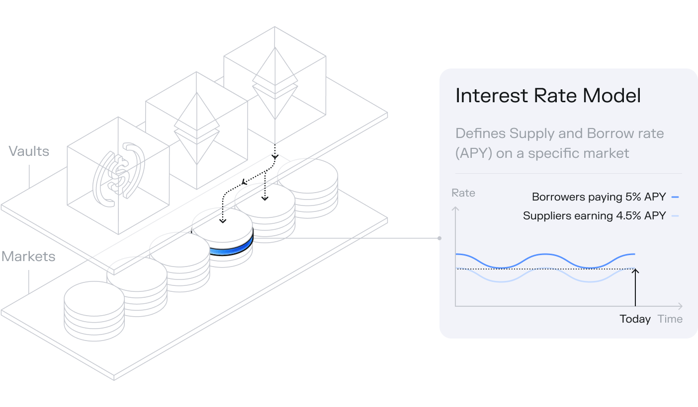
Morpho is an Interest Rate Model (IRM) agnostic protocol, meaning it can support any interest rate model for its markets. In Morpho, the interest borrowers pay in a given market is defined by the IRM chosen at market creation among a governance-approved set.

Initially, this set is composed of one immutable IRM, the AdaptiveCurveIRM.

The AdaptiveCurveIRM

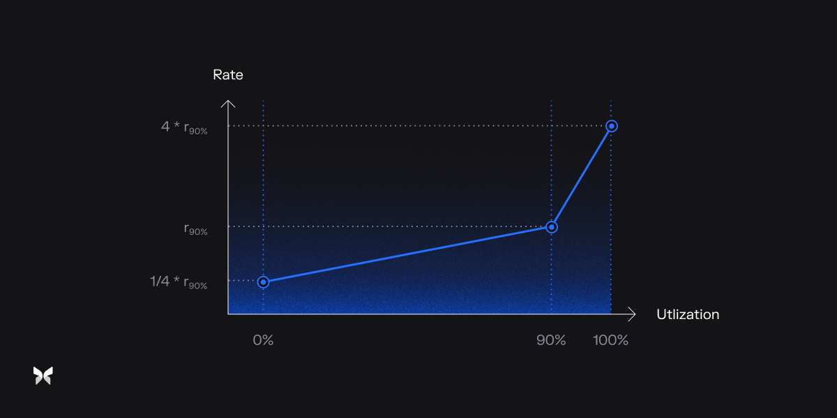
The AdaptiveCurveIRM is engineered to maintain the ratio of borrowed assets over supplied assets, commonly called utilization, close to a target of 90%.

In Morpho, the collateral supplied is not rehypothecated. Removing this systemic risk removes the liquidity constraints imposed by liquidation needs. It enables more efficient markets with higher target utilization of capital and lower penalties for illiquidity, resulting in better rates for both lenders and borrowers.

As with every parameter of a Morpho Market, the IRM address is immutable. This means that neither governance nor market creators can change it at any given time. As such, the AdaptiveCurveIRM is designed to adapt autonomously to market conditions, including changes in interest rates on other platforms and, more broadly, any shifts in supply and demand dynamics.

Its adaptability enables it to perform effectively across any asset, market, and condition, making it highly suitable for Morpho's permissionless market creation.

How It Works

The model can be broken down into two complementary mechanisms:

1. The Curve Mechanism This mechanism is akin to the interest rate curve in traditional lending pools. It manages short-term utilization effectively, maintaining capital efficiency while avoiding excessively high utilization zones that could lead to liquidity issues.

   

   $r_{90\%}$ is the target rate at utilization target $u_{target}=90\%$.

   Example with interest rate at 4% at $u_{target}$:

   • If utilization rate goes to 100% following a market event, the interest rate will instantly go to 4*$r_{90\%}$, 16% in this example.

   • At the opposite, if a market event bring the utilization rate to 0%, the utilization rate will instantly be $\frac{1}{4}$*$r_{90\%}$, 1% in this example.

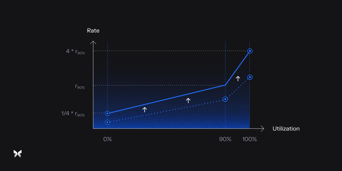
2. The Adaptive Mechanism This mechanism fine-tunes the curve over time to keep the range of rates in sync with market dynamics. It achieves this by adjusting the value of $r_{90\%}$, which in turn shifts the entire curve:

   • When utilization exceeds the target, the curve continuously shifts upward. This incentivizes loan repayment and thus decreases utilization.
   • When utilization falls below the target, the curve continuously shifts downward. This incentivizes borrowing and thus increases utilization.
   

   The speed at which the curve adjusts is determined by the distance of current utilization to the target: the further it is, the faster the curve shifts. This incremental adjustment of the curve allows for rate exploration, ultimately stabilizing when the interest rate at the target utilization aligns with the market equilibrium.

   Some examples are given below:

   • If the utilization remains at 45%, $r_{90\%}$ will progressively decrease until it is divided by 2 after 10 days.
   • If the utilization remains at 95%, $r_{90\%}$ will progressively increase until it doubles after 10 days.
   • If the utilization remains at 100%, $r_{90\%}$ will progressively increase until it doubles after 5 days. This is the maximum speed at which $r_{90\%}$ can move.

Here's a video showing how the two mechanisms combine to adjust interest rates:

For more on the AdaptiveCurveIRM, explore the technical reference.